Lazy beats Smart and Fast
Download as PPTX, PDF5 likes995 views

Julian Hyde's presentation at DataEngConf discusses optimizing SQL query performance through techniques like lazy evaluation, materialized views, and adaptive data systems using Apache Calcite. Key strategies include effective data organization, utilizing indexes, and implementing machine learning techniques for system tuning and query optimization. The focus is on improving query response time and resource utilization through intelligent data handling and self-optimizing systems.


![SELECT d.name, COUNT(*) AS c
FROM Emps AS e
JOIN Depts AS d USING (deptno)
WHERE e.age < 40
GROUP BY d.deptno
HAVING COUNT(*) > 5
ORDER BY c DESC
Relational algebra
Based on set theory, plus operators:
Project, Filter, Aggregate, Union, Join,
Sort
Requires: declarative language (SQL),
query planner
Original goal: data independence
Enables: query optimization, new
algorithms and data structures
Scan [Emps] Scan [Depts]
Join [e.deptno = d.deptno]
Filter [e.age < 30]
Aggregate [deptno, COUNT(*) AS c]
Filter [c > 5]
Project [name, c]
Sort [c DESC]](https://image.slidesharecdn.com/calcite-data-eng-2018-180417212904/85/Lazy-beats-Smart-and-Fast-8-320.jpg)


![Materialized view
CREATE MATERIALIZED
VIEW EmpsByDeptno AS
SELECT deptno, name, deptno
FROM Emp
ORDER BY deptno, name;
Scan [Emps]
Scan [EmpsByDeptno]
Sort [deptno, name]
empno name deptno
100 Fred 20
110 Barney 10
120 Wilma 30
130 Dino 10
deptno name empno
10 Barney 100
10 Dino 130
20 Fred 20
30 Wilma 30
As a materialized view, an
index is now just another
table
Several tables contain the
information necessary to
answer the query - just pick
the best](https://image.slidesharecdn.com/calcite-data-eng-2018-180417212904/85/Lazy-beats-Smart-and-Fast-14-320.jpg)


![Algorithm: Design summary tables
Given a database with 30 columns, 10M rows. Find X summary tables with under
Y rows that improve query response time the most.
AdaptiveMonteCarlo algorithm [1]:
● Based on research [2]
● Greedy algorithm that takes a combination of summary tables and tries to
find the table that yields the greatest cost/benefit improvement
● Models “benefit” of the table as query time saved over simulated query load
● The “cost” of a table is its size
[1] org.pentaho.aggdes.algorithm.impl.AdaptiveMonteCarloAlgorithm
[2] Harinarayan, Rajaraman, Ullman (1996). “Implementing data cubes efficiently”](https://image.slidesharecdn.com/calcite-data-eng-2018-180417212904/85/Lazy-beats-Smart-and-Fast-28-320.jpg)
![Data profiling
Algorithm needs count(distinct a, b, ...) for each combination of attributes:
● Previous example had 25 = 32 possible tables
● Schema with 30 attributes has 230 (about 109) possible tables
● Algorithm considers a significant fraction of these
● Approximations are OK
Attempts to solve the profiling problem:
1. Compute each combination: scan, sort, unique, count; repeat 230 times!
2. Sketches (HyperLogLog)
3. Sketches + parallelism + information theory [CALCITE-1616]](https://image.slidesharecdn.com/calcite-data-eng-2018-180417212904/85/Lazy-beats-Smart-and-Fast-30-320.jpg)
![Sketches
HyperLogLog is an algorithm that computes
approximate distinct count. It can estimate
cardinalities of 109 with a typical error rate of
2%, using 1.5 kB of memory. [3][4]
With 16 MB memory per machine we can
compute 10,000 combinations of attributes
each pass.
So, we’re down from 109 to 105 passes.
[3] Flajolet, Fusy, Gandouet, Meunier (2007). "Hyperloglog: The analysis of a near-optimal cardinality estimation algorithm"
[4] https://github.com/mrjgreen/HyperLogLog](https://image.slidesharecdn.com/calcite-data-eng-2018-180417212904/85/Lazy-beats-Smart-and-Fast-31-320.jpg)
![Lattice after Query 1 + 2
Query 2
Query 1
Growing and evolving
lattices based on queries
sales
customers
product
product
class
sales
product
product
class
sales
customers
See: [CALCITE-1870] “Lattice suggester”](https://image.slidesharecdn.com/calcite-data-eng-2018-180417212904/85/Lazy-beats-Smart-and-Fast-38-320.jpg)
![Thank you! Questions?
@julianhyde | @ApacheCalcite | http://apache.calcite.org
Resources
[CALCITE-1616] Data profiler
[CALCITE-1870] Lattice suggester
[CALCITE-1861] Spatial indexes
[CALCITE-1968] OpenGIS
[CALCITE-1991] Generated columns
Talk: “Data profiling with Apache Calcite” (Hadoop Summit, 2017)
Talk: “SQL on everything, in memory” (Strata, 2014)
Zhang, Qi, Stradling, Huang (2014). “Towards a Painless Index for Spatial Objects”
Harinarayan, Rajaraman, Ullman (1996). “Implementing data cubes efficiently”
Image credit
https://www.flickr.com/photos/defenceimages/6938469933/](https://image.slidesharecdn.com/calcite-data-eng-2018-180417212904/85/Lazy-beats-Smart-and-Fast-40-320.jpg)


Lazy beats Smart and Fast
- 1. Lazy beats Smart & Fast Julian Hyde | DataEngConf SF 2018/04/17
- 2. @julianhyde SQL Query planning Query federation OLAP Streaming Hadoop ASF member Original author of Apache Calcite PMC Apache Arrow, Calcite, Drill, Eagle, Kylin Architect at Looker
- 4. A “simple” query Data ● 2010 U.S. census ● 100 million records ● 1KB per record ● 100 GB total System ● 4x SATA 3 disks ● Total read throughput 1 GB/s Query Goal ● Compute the answer to the query in under 5 seconds SELECT SUM(householdSize) FROM CensusHouseholds;
- 5. Solutions Sequential scan Query takes 100 s (100 GB at 1 GB/s) Parallelize Spread the data over 40 disks in 10 machines Query takes 10 s Cache Keep the data in memory 2nd query: 10 ms 3rd query: 10 s Materialize Summarize the data on disk All queries: 100 ms Materialize + cache + adapt As above, building summaries on demand
- 6. Lazy > Smart + Fast (Lazy + adaptive is even better)
- 7. Overview How do you tune a data system? How can (or should) a data system tune itself? What problems have we solved to bring these things to Apache Calcite? Part 1: Strategies for organizing data Part 2: How to make systems self-organizing?
- 8. SELECT d.name, COUNT(*) AS c FROM Emps AS e JOIN Depts AS d USING (deptno) WHERE e.age < 40 GROUP BY d.deptno HAVING COUNT(*) > 5 ORDER BY c DESC Relational algebra Based on set theory, plus operators: Project, Filter, Aggregate, Union, Join, Sort Requires: declarative language (SQL), query planner Original goal: data independence Enables: query optimization, new algorithms and data structures Scan [Emps] Scan [Depts] Join [e.deptno = d.deptno] Filter [e.age < 30] Aggregate [deptno, COUNT(*) AS c] Filter [c > 5] Project [name, c] Sort [c DESC]
- 9. Apache Calcite Apache top-level project Query planning framework used in many projects and products Also works standalone: embedded federated query engine with SQL / JDBC front end Apache community development model http://calcite.apache.org http://github.com/apache/calcite
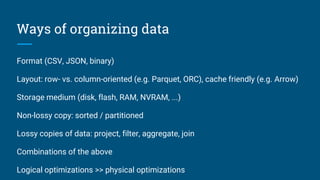
- 11. Ways of organizing data Format (CSV, JSON, binary) Layout: row- vs. column-oriented (e.g. Parquet, ORC), cache friendly (e.g. Arrow) Storage medium (disk, flash, RAM, NVRAM, ...) Non-lossy copy: sorted / partitioned Lossy copies of data: project, filter, aggregate, join Combinations of the above Logical optimizations >> physical optimizations
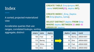
- 12. Index A sorted, projected materialized view Accelerates queries that use ranges, correlated lookups, sorting, aggregate, distinct CREATE TABLE Emp (empno INT, name VARCHAR(20), deptno INT); CREATE INDEX I_Emp_Deptno ON Emp (deptno, name); SELECT DISTINCT deptno FROM Emp WHERE deptno BETWEEN 20 AND 40 ORDER BY deptno; empno name deptno 100 Fred 20 110 Barney 10 120 Wilma 30 130 Dino 10 deptno name rowid 10 Barney af5634.0001 10 Dino af5634.0003 20 Fred af5634.0000 30 Wilma af5634.0002
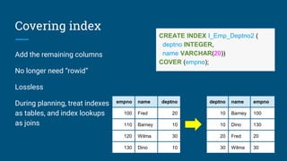
- 13. Add the remaining columns No longer need “rowid” Lossless During planning, treat indexes as tables, and index lookups as joins Covering index empno name deptno 100 Fred 20 110 Barney 10 120 Wilma 30 130 Dino 10 deptno name empno 10 Barney 100 10 Dino 130 20 Fred 20 30 Wilma 30 CREATE INDEX I_Emp_Deptno2 ( deptno INTEGER, name VARCHAR(20)) COVER (empno);
- 14. Materialized view CREATE MATERIALIZED VIEW EmpsByDeptno AS SELECT deptno, name, deptno FROM Emp ORDER BY deptno, name; Scan [Emps] Scan [EmpsByDeptno] Sort [deptno, name] empno name deptno 100 Fred 20 110 Barney 10 120 Wilma 30 130 Dino 10 deptno name empno 10 Barney 100 10 Dino 130 20 Fred 20 30 Wilma 30 As a materialized view, an index is now just another table Several tables contain the information necessary to answer the query - just pick the best
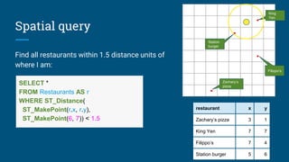
- 15. Spatial query Find all restaurants within 1.5 distance units of where I am: restaurant x y Zachary’s pizza 3 1 King Yen 7 7 Filippo’s 7 4 Station burger 5 6 SELECT * FROM Restaurants AS r WHERE ST_Distance( ST_MakePoint(r.x, r.y), ST_MakePoint(6, 7)) < 1.5 • • • • Zachary’s pizza Filippo’s King Yen Station burger
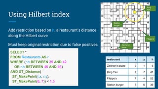
- 16. Hilbert space-filling curve ● A space-filling curve invented by mathematician David Hilbert ● Every (x, y) point has a unique position on the curve ● Points near to each other typically have Hilbert indexes close together
- 17. • • • • Add restriction based on h, a restaurant’s distance along the Hilbert curve Must keep original restriction due to false positives Using Hilbert index restaurant x y h Zachary’s pizza 3 1 5 King Yen 7 7 41 Filippo’s 7 4 52 Station burger 5 6 36 Zachary’s pizza Filippo’s SELECT * FROM Restaurants AS r WHERE (r.h BETWEEN 35 AND 42 OR r.h BETWEEN 46 AND 46) AND ST_Distance( ST_MakePoint(r.x, r.y), ST_MakePoint(6, 7)) < 1.5 King Yen Station burger
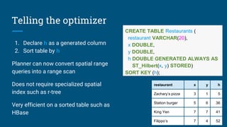
- 18. Telling the optimizer 1. Declare h as a generated column 2. Sort table by h Planner can now convert spatial range queries into a range scan Does not require specialized spatial index such as r-tree Very efficient on a sorted table such as HBase CREATE TABLE Restaurants ( restaurant VARCHAR(20), x DOUBLE, y DOUBLE, h DOUBLE GENERATED ALWAYS AS ST_Hilbert(x, y) STORED) SORT KEY (h); restaurant x y h Zachary’s pizza 3 1 5 Station burger 5 6 36 King Yen 7 7 41 Filippo’s 7 4 52
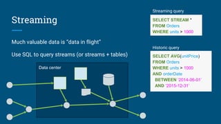
- 19. Much valuable data is “data in flight” Use SQL to query streams (or streams + tables) Streaming Data center SELECT AVG(unitPrice) FROM Orders WHERE units > 1000 AND orderDate BETWEEN ‘2014-06-01’ AND ‘2015-12-31’ SELECT STREAM * FROM Orders WHERE units > 1000 Streaming query Historic query
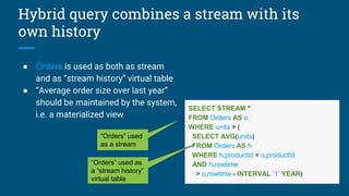
- 20. Hybrid query combines a stream with its own history ● Orders is used as both as stream and as “stream history” virtual table ● “Average order size over last year” should be maintained by the system, i.e. a materialized view SELECT STREAM * FROM Orders AS o WHERE units > ( SELECT AVG(units) FROM Orders AS h WHERE h.productId = o.productId AND h.rowtime > o.rowtime - INTERVAL ‘1’ YEAR) “Orders” used as a stream “Orders” used as a “stream history” virtual table
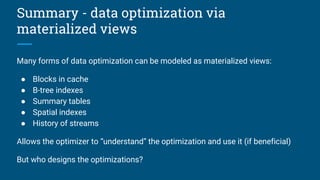
- 21. Summary - data optimization via materialized views Many forms of data optimization can be modeled as materialized views: ● Blocks in cache ● B-tree indexes ● Summary tables ● Spatial indexes ● History of streams Allows the optimizer to “understand” the optimization and use it (if beneficial) But who designs the optimizations?
- 22. 2. Learning
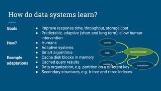
- 23. How do data systems learn? queries DML statistics adaptations recommender Goals ● Improve response time, throughput, storage cost ● Predictable, adaptive (short and long term), allow human intervention How? ● Humans ● Adaptive systems ● Smart algorithms Example adaptations ● Cache disk blocks in memory ● Cached query results ● Data organization, e.g. partition on a different key ● Secondary structures, e.g. b-tree and r-tree indexes
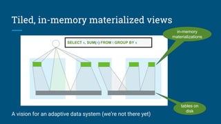
- 24. Tiled, in-memory materialized views A vision for an adaptive data system (we’re not there yet) tables on disk in-memory materializations SELECT x, SUM(n) FROM t GROUP BY x
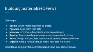
- 25. Building materialized views Challenges: ● Design Which materializations to create? ● Populate Load them with data ● Maintain Incrementally populate when data changes ● Rewrite Transparently rewrite queries to use materializations ● Adapt Design and populate new materializations, drop unused ones ● Express Need a rich algebra, to model how data is derived Initial focus: summary tables (materialized views over star schemas)
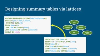
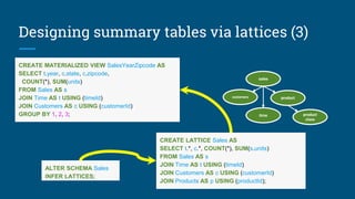
- 26. CREATE LATTICE Sales AS SELECT t.*, c.*, COUNT(*), SUM(s.units) FROM Sales AS s JOIN Time AS t USING (timeId) JOIN Customers AS c USING (customerId) JOIN Products AS p USING (productId); Designing summary tables via lattices CREATE MATERIALIZED VIEW SalesYearZipcode AS SELECT t.year, c.state, c.zipcode, COUNT(*), SUM(units) FROM Sales AS s JOIN Time AS t USING (timeId) JOIN Customers AS c USING (customerId) GROUP BY 1, 2, 3; product product class sales customers time
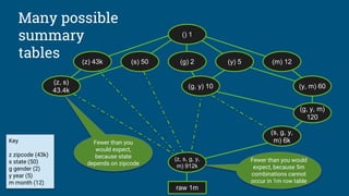
- 27. Many possible summary tables Key z zipcode (43k) s state (50) g gender (2) y year (5) m month (12) () 1 (z, s, g, y, m) 912k (s, g, y, m) 6k (z) 43k (s) 50 (g) 2 (y) 5 (m) 12 raw 1m (y, m) 60(g, y) 10 (z, s) 43.4k (g, y, m) 120 Fewer than you would expect, because 5m combinations cannot occur in 1m row table Fewer than you would expect, because state depends on zipcode
- 28. Algorithm: Design summary tables Given a database with 30 columns, 10M rows. Find X summary tables with under Y rows that improve query response time the most. AdaptiveMonteCarlo algorithm [1]: ● Based on research [2] ● Greedy algorithm that takes a combination of summary tables and tries to find the table that yields the greatest cost/benefit improvement ● Models “benefit” of the table as query time saved over simulated query load ● The “cost” of a table is its size [1] org.pentaho.aggdes.algorithm.impl.AdaptiveMonteCarloAlgorithm [2] Harinarayan, Rajaraman, Ullman (1996). “Implementing data cubes efficiently”
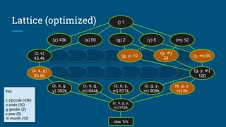
- 29. Lattice (optimized) () 1 (z, s, g, y, m) 912k (s, g, y, m) 6k (z) 43k (s) 50 (g) 2 (y) 5 (m) 12 (z, g, y, m) 909k (z, s, y, m) 831k raw 1m (z, s, g, m) 644k (z, s, g, y) 392k (y, m) 60 (z, s) 43.4k (z, s, g) 83.6k (g, y) 10 (g, y, m) 120 (g, m) 24 Key z zipcode (43k) s state (50) g gender (2) y year (5) m month (12)
- 30. Data profiling Algorithm needs count(distinct a, b, ...) for each combination of attributes: ● Previous example had 25 = 32 possible tables ● Schema with 30 attributes has 230 (about 109) possible tables ● Algorithm considers a significant fraction of these ● Approximations are OK Attempts to solve the profiling problem: 1. Compute each combination: scan, sort, unique, count; repeat 230 times! 2. Sketches (HyperLogLog) 3. Sketches + parallelism + information theory [CALCITE-1616]
- 31. Sketches HyperLogLog is an algorithm that computes approximate distinct count. It can estimate cardinalities of 109 with a typical error rate of 2%, using 1.5 kB of memory. [3][4] With 16 MB memory per machine we can compute 10,000 combinations of attributes each pass. So, we’re down from 109 to 105 passes. [3] Flajolet, Fusy, Gandouet, Meunier (2007). "Hyperloglog: The analysis of a near-optimal cardinality estimation algorithm" [4] https://github.com/mrjgreen/HyperLogLog
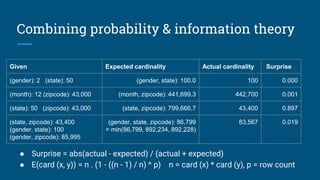
- 32. Given Expected cardinality Actual cardinality Surprise (gender): 2 (state): 50 (gender, state): 100.0 100 0.000 (month): 12 (zipcode): 43,000 (month, zipcode): 441,699.3 442,700 0.001 (state): 50 (zipcode): 43,000 (state, zipcode): 799,666.7 43,400 0.897 (state, zipcode): 43,400 (gender, state): 100 (gender, zipcode): 85,995 (gender, state, zipcode): 86,799 = min(86,799, 892,234, 892,228) 83,567 0.019 ● Surprise = abs(actual - expected) / (actual + expected) ● E(card (x, y)) = n . (1 - ((n - 1) / n) ^ p) n = card (x) * card (y), p = row count Combining probability & information theory
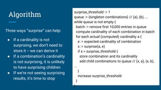
- 33. Algorithm Three ways “surprise” can help: ● If a cardinality is not surprising, we don’t need to store it -- we can derive it ● If a combination’s cardinality is not surprising, it is unlikely to have surprising children ● If we’re not seeing surprising results, it’s time to stop surprise_threshold := 1 queue := {singleton combinations} // (a), (b), ... while queue is not empty { batch := remove first 10,000 entries in queue compute cardinality of each combination in batch for each actual (computed) cardinality a { e := expected cardinality of combination s := surprise(a, e) if s > surprise_threshold { store combination and its cardinality add child combinations to queue // (x, a), (x, b), ... } increase surprise_threshold } }
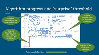
- 34. Algorithm progress and “surprise” threshold Progress of algorithm Rejected as not sufficiently surprising Surprise threshold rises as algorithm progresses Singleton combinations are have surprise = 1 Surprise threshold rises after we have completed the first batch
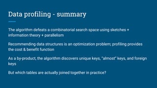
- 35. Data profiling - summary The algorithm defeats a combinatorial search space using sketches + information theory + parallelism Recommending data structures is an optimization problem; profiling provides the cost & benefit function As a by-product, the algorithm discovers unique keys, “almost” keys, and foreign keys But which tables are actually joined together in practice?
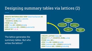
- 36. CREATE LATTICE Sales AS SELECT t.*, c.*, COUNT(*), SUM(s.units) FROM Sales AS s JOIN Time AS t USING (timeId) JOIN Customers AS c USING (customerId) JOIN Products AS p USING (productId); CREATE MATERIALIZED VIEW SalesYearZipcode AS SELECT t.year, c.state, c.zipcode, COUNT(*), SUM(units) FROM Sales AS s JOIN Time AS t USING (timeId) JOIN Customers AS c USING (customerId) GROUP BY 1, 2, 3; product product class sales customers time The lattice generates the summary tables. But who writes the lattice? Designing summary tables via lattices (2)
- 37. CREATE LATTICE Sales AS SELECT t.*, c.*, COUNT(*), SUM(s.units) FROM Sales AS s JOIN Time AS t USING (timeId) JOIN Customers AS c USING (customerId) JOIN Products AS p USING (productId); CREATE MATERIALIZED VIEW SalesYearZipcode AS SELECT t.year, c.state, c.zipcode, COUNT(*), SUM(units) FROM Sales AS s JOIN Time AS t USING (timeId) JOIN Customers AS c USING (customerId) GROUP BY 1, 2, 3; ALTER SCHEMA Sales INFER LATTICES; product product class sales customers time Designing summary tables via lattices (3)
- 38. Lattice after Query 1 + 2 Query 2 Query 1 Growing and evolving lattices based on queries sales customers product product class sales product product class sales customers See: [CALCITE-1870] “Lattice suggester”
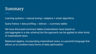
- 39. Summary Learning systems = manual tuning + adaptive + smart algorithms Query history + data profiling→ lattices → summary tables We have discussed summary tables (materialized views based on join/aggregate in a star schema) but the approach can be applied to other kinds of materialized views Relational algebra, incorporating materialized views, is a powerful language that allows us to combine many forms of data optimization
- 40. Thank you! Questions? @julianhyde | @ApacheCalcite | http://apache.calcite.org Resources [CALCITE-1616] Data profiler [CALCITE-1870] Lattice suggester [CALCITE-1861] Spatial indexes [CALCITE-1968] OpenGIS [CALCITE-1991] Generated columns Talk: “Data profiling with Apache Calcite” (Hadoop Summit, 2017) Talk: “SQL on everything, in memory” (Strata, 2014) Zhang, Qi, Stradling, Huang (2014). “Towards a Painless Index for Spatial Objects” Harinarayan, Rajaraman, Ullman (1996). “Implementing data cubes efficiently” Image credit https://www.flickr.com/photos/defenceimages/6938469933/
- 42. Extra slides
- 44. Planning queries MySQL Splunk join Key: productId group Key: productName Agg: count filter Condition: action = 'purchase' sort Key: c desc scan scan Table: products select p.productName, count(*) as c from splunk.splunk as s join mysql.products as p on s.productId = p.productId where s.action = 'purchase' group by p.productName order by c desc Table: splunk
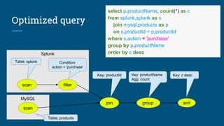
- 45. Optimized query MySQL Splunk join Key: productId group Key: productName Agg: count filter Condition: action = 'purchase' sort Key: c desc scan scan Table: splunk Table: products select p.productName, count(*) as c from splunk.splunk as s join mysql.products as p on s.productId = p.productId where s.action = 'purchase' group by p.productName order by c desc
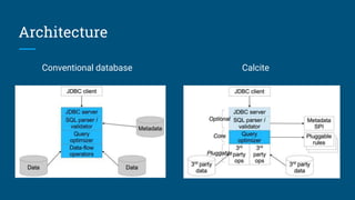
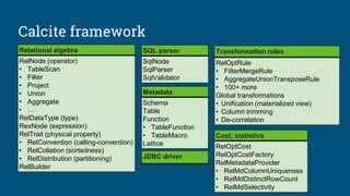
- 46. Calcite framework Cost, statistics RelOptCost RelOptCostFactory RelMetadataProvider • RelMdColumnUniquensss • RelMdDistinctRowCount • RelMdSelectivity SQL parser SqlNode SqlParser SqlValidator Transformation rules RelOptRule • FilterMergeRule • AggregateUnionTransposeRule • 100+ more Global transformations • Unification (materialized view) • Column trimming • De-correlation Relational algebra RelNode (operator) • TableScan • Filter • Project • Union • Aggregate • … RelDataType (type) RexNode (expression) RelTrait (physical property) • RelConvention (calling-convention) • RelCollation (sortedness) • RelDistribution (partitioning) RelBuilder JDBC driver Metadata Schema Table Function • TableFunction • TableMacro Lattice
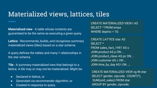
- 47. Materialized views, lattices, tiles Materialized view - A table whose contents are guaranteed to be the same as executing a given query. Lattice - Recommends, builds, and recognizes summary materialized views (tiles) based on a star schema. A query defines the tables and many:1 relationships in the star schema. Tile - A summary materialized view that belongs to a lattice. A tile may or may not be materialized. Might be: ● Declared in lattice, or ● Generated via recommender algorithm, or ● Created in response to query. CREATE MATERIALIZED VIEW t AS SELECT * FROM emps WHERE deptno = 10; CREATE LATTICE star AS SELECT * FROM sales_fact_1997 AS s JOIN product AS p ON … JOIN product_class AS pc ON … JOIN customer AS c ON … JOIN time_by_day AS t ON …; CREATE MATERIALIZED VIEW zg IN star SELECT gender, zipcode, COUNT(*), SUM(unit_sales) FROM star GROUP BY gender, zipcode;
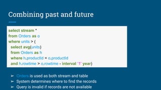
- 48. Combining past and future select stream * from Orders as o where units > ( select avg(units) from Orders as h where h.productId = o.productId and h.rowtime > o.rowtime - interval ‘1’ year) ➢ Orders is used as both stream and table ➢ System determines where to find the records ➢ Query is invalid if records are not available
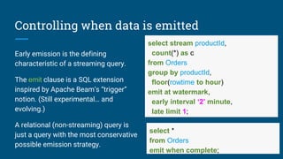
- 49. Controlling when data is emitted Early emission is the defining characteristic of a streaming query. The emit clause is a SQL extension inspired by Apache Beam’s “trigger” notion. (Still experimental… and evolving.) A relational (non-streaming) query is just a query with the most conservative possible emission strategy. select stream productId, count(*) as c from Orders group by productId, floor(rowtime to hour) emit at watermark, early interval ‘2’ minute, late limit 1; select * from Orders emit when complete;
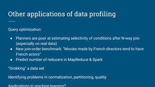
- 50. Other applications of data profiling Query optimization: ● Planners are poor at estimating selectivity of conditions after N-way join (especially on real data) ● New join-order benchmark: “Movies made by French directors tend to have French actors” ● Predict number of reducers in MapReduce & Spark “Grokking” a data set Identifying problems in normalization, partitioning, quality
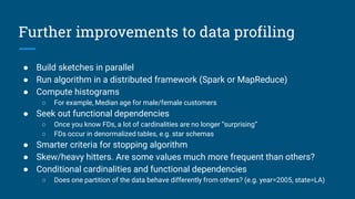
- 51. Further improvements to data profiling ● Build sketches in parallel ● Run algorithm in a distributed framework (Spark or MapReduce) ● Compute histograms ○ For example, Median age for male/female customers ● Seek out functional dependencies ○ Once you know FDs, a lot of cardinalities are no longer “surprising” ○ FDs occur in denormalized tables, e.g. star schemas ● Smarter criteria for stopping algorithm ● Skew/heavy hitters. Are some values much more frequent than others? ● Conditional cardinalities and functional dependencies ○ Does one partition of the data behave differently from others? (e.g. year=2005, state=LA)
Editor's Notes
- #4: I recently joined Looker. Looker is a data platform. It allows everyone in the company to get at their data, and everyone sees a consistent view. Business users love looker because they can get at what they need without writing SQL. Operations folks love looker because the data model is based on code that humans can read, write, commit to git, diff, and merge. Customers love Looker. Employees love working at Looker. We are hiring.
- #5: To motivate, let’s look at a simple problem. Which may not be so simple. Not for any particular database - we’re talking about the laws of physics here. An analytic query - figure out the number of people in the country Impossible to meet the goal - it takes 80 seconds to read the data One possible solution is to buy 100 GB of memory. Another is to buy another 80 disks.
- #6: Parallel scan = fast Caching = smart Using materializations = lazy
- #8: What I am going to talk about today is old knowledge Query optimization (I prefer to call it planning) relies on relational algebra - a declarative query language, and a mathematically sound way of transforming queries to We’ll look at what relational algebra can do for the related problem of how to organize the data for efficient query There is talk of “self-driving database” Part 1. How to organize data? We rely heavily on relational algebra, especially materialized views. Part 2: How to make systems self-organizing? (Algorithms for design materialized views, infer relationships between data sets, gathering statistics about data sets.)
- #9: The main “very old idea” in this talk is relational algebra. As you know it enables query optimization, but it also enables data optimization Based on set theory -- albeit sets that allow duplicates and in some cases have a defined order Users write their queries in a declarative language - with the understanding that they will be The original motivation was to avoid putting disk block addresses in data sets. Allowed us to move the data to a different disk without re-writing it. Data became logical. But once we have an optimizer, the optimizer can choose algorithms and can accept new data structures, without changing the query Enables query optimization, new algorithms (e.g. hash join, merge join), new data structures (e.g. r-trees, sorted partitions), abstraction (e.g. views), security (e.g. access-controlled views)
- #10: Our typical contributors are members of other projects, say Hive or Flink. They contribute the extensions to the framework that they need. MapD (database on GPUs) just went open source.
- #12: When choosing how to organize data, there are many dimensions. But the logical optimizations deliver orders of magnitude improvements. Data format - e.g. CSV if textual, various binary formats; the more schema is known in advance, the more concise the format can be A simple copy of data is a snapshot. Useful if it provides redundancy, but more useful if it has different sort / partitioning If two tables are partitioned or sorted on the same key, they can be more easily joined Choosing the right
- #13: Let’s look at the oldest and still most popular data structure for optimizing data We’re all familiar with indexes. Indexes made relational databases practical in the mid-70s Did you know that an index is a materialized view? Technically it’s, a sorted, projected materialized view, duplicates retained
- #14: Let’s look at a slightly different kind of index. It is still sorted, which gives us the same advantages for range queries and so forth. It doesn’t contain rowids, because in analytic databases random IOs are too expensive. Pure relational, loss-less MV puts it on sound algebraic footing
- #15: Same data structure as previously, but represented generically It doesn’t contain rowids, because in analytic databases random IOs are too expensive. Pure relational, loss-less MV puts it on sound algebraic footing
- #16: Calcite recently added OpenGIS extensions to SQL standard
- #17: Here are 3 generations of generating the Hilbert curve. You can go on… every point has a position on the curve. I actually prefer to think of the Hilbert index as a binary fraction between 0 and 1. It is a permutation and interleaving of the bits of the (x, y) coordinates. Dimension reduction from 2 to 1 dimensions means we can use b-tree indexes, range partitions etc.
- #21: This query combines both future (stream) and past. The past is useful to automatically normalize data, and figure out what is ‘exceptional’ without involving a human. “Any useful metric is dimensionless” (in the physics sense, i.e. it has no units, because it is a ratio) The system determines where to find the historical and streaming records. The records might be available in more than one place (in which case the system adds value by choosing the best) or nowhere (in which case the query is invalid because it is unsatisfiable).
- #24: Over time, the data changes (usually grows), and users run queries The main agent tuning the system is -- for now at least -- humans. Database administrators observe the data and the query load and optimize the system. Improve understanding of the system Gather statistics -- e.g. ANALYZE TABLE, deduce unique and foreign keys Observe query patterns Observe how data is loaded (e.g. is a table read-only, append-only) Inputs the recommender are queries, the pattern of DML activity (inserts, updates, deletes), and data volumetrics; outputs are recommended adaptations (e.g. summary tables to build). Iterate, because if you build a summary table it might reduce load on another part of the system
- #25: Where we’d like to go is in-memory materializations. Adaptive and in-memory (like cache) but summarized (like summary tables) therefore more compact. Unlike cache, is known to the planner. Some most of the data needed by the query is in memory in summarized “tiles”. Possibly created by previous queries. Where there are gaps, the query goes to disk, but it can still answer the query. Over time the useful data ends up in memory.
- #29: Algorithm just needs to know how many rows each summary table would contain. Compute count(distinct x, y, z) for each combination of attributes. Full scan, sort, unique, count; repeat 230 times But there are 230 possible summary tables!
- #35: We don’t store results that are not “surprising” We don’t explore children of un-surprising combinations of attributes
- #36: Recommending data structures is an optimization problem.
- #46: Two rules have fired, filter-join-transpose-rule followed by splunk-filter-rule, and the query has become more efficient, because many fewer rows are coming out of Splunk. To truly optimize the query we would need to fire many more rules, and apply a cost model to choose which of the many equivalent plans is the best.
- #49: This query combines both future (stream) and past. The past is useful to automatically normalize data, and figure out what is ‘exceptional’ without involving a human. “Any useful metric is dimensionless” (in the physics sense, i.e. it has no units, because it is a ratio) The system determines where to find the historical and streaming records. The records might be available in more than one place (in which case the system adds value by choosing the best) or nowhere (in which case the query is invalid because it is unsatisfiable).
- #51: Maybe that “almost hierarchy” should be a true hierarchy -- so you have a quality problem If attributes have a lower cardinality than expected, then maybe you can use one to predict another